Testing covariate modelling in hierarchical parent degradation kinetics with residue data on mesotrione

Introduction

The purpose of this document is to test demonstrate how nonlinear hierarchical models (NLHM) based on the parent degradation models SFO, FOMC, DFOP and HS can be fitted with the mkin package, also considering the influence of covariates like soil pH on different degradation parameters. Because in some other case studies, the SFORB parameterisation of biexponential decline has shown some advantages over the DFOP parameterisation, SFORB was included in the list of tested models as well.

The mkin package is used in version 1.2.6, which is contains the functions that were used for the evaluations. The saemix package is used as a backend for fitting the NLHM, but is also loaded to make the convergence plot function available.

This document is processed with the knitr package, which also provides the kable function that is used to improve the display of tabular data in R markdown documents. For parallel processing, the parallel package is used.

library(mkin)
library(knitr)
library(saemix)
library(parallel)
n_cores <- detectCores()
if (Sys.info()["sysname"] == "Windows") {
  cl <- makePSOCKcluster(n_cores)
} else {
  cl <- makeForkCluster(n_cores)
}

Test data

data_file <- system.file(
  "testdata", "mesotrione_soil_efsa_2016.xlsx", package = "mkin")
meso_ds <- read_spreadsheet(data_file, parent_only = TRUE)

The following tables show the covariate data and the 18 datasets that were read in from the spreadsheet file.

pH <- attr(meso_ds, "covariates")
kable(pH, caption = "Covariate data")

Covariate data
	pH
Richmond	6.2
Richmond 2	6.2
ERTC	6.4
Toulouse	7.7
Picket Piece	7.1
721	5.6
722	5.7
723	5.4
724	4.8
725	5.8
727	5.1
728	5.9
729	5.6
730	5.3
731	6.1
732	5.0
741	5.7
742	7.2

for (ds_name in names(meso_ds)) {
  print(
    kable(mkin_long_to_wide(meso_ds[[ds_name]]),
      caption = paste("Dataset", ds_name),
      booktabs = TRUE, row.names = FALSE))
}

Dataset Richmond
time	meso
0.000000	91.00
1.179050	86.70
3.537149	73.60
7.074299	61.50
10.611448	55.70
15.327647	47.70
17.685747	39.50
24.760046	29.80
35.371494	19.60
68.384889	5.67
0.000000	97.90
1.179050	96.40
3.537149	89.10
7.074299	74.40
10.611448	57.40
15.327647	46.30
18.864797	35.50
27.118146	27.20
35.371494	19.10
74.280138	6.50
108.472582	3.40
142.665027	2.20

Dataset Richmond 2
time	meso
0.000000	96.0
2.422004	82.4
5.651343	71.2
8.073348	53.1
11.302687	48.5
16.954030	33.4
22.605373	24.2
45.210746	11.9

Dataset ERTC
time	meso
0.000000	99.9
2.755193	80.0
6.428782	42.1
9.183975	50.1
12.857565	28.4
19.286347	39.8
25.715130	29.9
51.430259	2.5

Dataset Toulouse
time	meso
0.000000	96.8
2.897983	63.3
6.761960	22.3
9.659942	16.6
13.523919	16.1
20.285879	17.2
27.047838	1.8

Dataset Picket Piece
time	meso
0.000000	102.0
2.841195	73.7
6.629454	35.5
9.470649	31.8
13.258909	18.0
19.888364	3.7

Dataset 721
time	meso
0.00000	86.4
11.24366	61.4
22.48733	49.8
33.73099	41.0
44.97466	35.1

Dataset 722
time	meso
0.00000	90.3
11.24366	52.1
22.48733	37.4
33.73099	21.2
44.97466	14.3

Dataset 723
time	meso
0.00000	89.3
11.24366	70.8
22.48733	51.1
33.73099	42.7
44.97466	26.7

Dataset 724
time	meso
0.000000	89.4
9.008208	65.2
18.016415	55.8
27.024623	46.0
36.032831	41.7

Dataset 725
time	meso
0.00000	89.0
10.99058	35.4
21.98116	18.6
32.97174	11.6
43.96232	7.6

Dataset 727
time	meso
0.00000	91.3
10.96104	63.2
21.92209	51.1
32.88313	42.0
43.84417	40.8

Dataset 728
time	meso
0.00000	91.8
11.24366	43.6
22.48733	22.0
33.73099	15.9
44.97466	8.8

Dataset 729
time	meso
0.00000	91.6
11.24366	60.5
22.48733	43.5
33.73099	28.4
44.97466	20.5

Dataset 730
time	meso
0.00000	92.7
11.07446	58.9
22.14893	44.0
33.22339	46.0
44.29785	29.3

Dataset 731
time	meso
0.00000	92.1
11.24366	64.4
22.48733	45.3
33.73099	33.6
44.97466	23.5

Dataset 732
time	meso
0.00000	90.3
11.24366	58.2
22.48733	40.1
33.73099	33.1
44.97466	25.8

Dataset 741
time	meso
0.00000	90.3
10.84712	68.7
21.69424	58.0
32.54136	52.2
43.38848	48.0

Dataset 742
time	meso
0.00000	92.0
11.24366	60.9
22.48733	36.2
33.73099	18.3
44.97466	8.7

Separate evaluations

In order to obtain suitable starting parameters for the NLHM fits, separate fits of the five models to the data for each soil are generated using the mmkin function from the mkin package. In a first step, constant variance is assumed. Convergence is checked with the status function.

deg_mods <- c("SFO", "FOMC", "DFOP", "SFORB", "HS")
f_sep_const <- mmkin(
  deg_mods,
  meso_ds,
  error_model = "const",
  cluster = cl,
  quiet = TRUE)

status(f_sep_const[, 1:5]) |> kable()

	Richmond	Richmond 2	ERTC	Toulouse	Picket Piece
SFO	OK	OK	OK	OK	OK
FOMC	OK	OK	OK	OK	C
DFOP	OK	OK	OK	OK	OK
SFORB	OK	OK	OK	OK	OK
HS	OK	OK	C	OK	OK

status(f_sep_const[, 6:18]) |> kable()

	721	722	723	724	725	727	728	729	730	731	732	741	742
SFO	OK	OK	OK	OK	OK	OK	OK	OK	OK	OK	OK	OK	OK
FOMC	OK	OK	C	OK	OK	OK	OK	OK	OK	OK	OK	OK	OK
DFOP	OK	OK	OK	OK	OK	OK	OK	OK	OK	OK	OK	OK	OK
SFORB	OK	OK	OK	OK	OK	OK	OK	C	OK	OK	OK	OK	OK
HS	OK	OK	OK	OK	OK	OK	OK	OK	OK	OK	OK	OK	OK

In the tables above, OK indicates convergence and C indicates failure to converge. Most separate fits with constant variance converged, with the exception of two FOMC fits, one SFORB fit and one HS fit.

f_sep_tc <- update(f_sep_const, error_model = "tc")

status(f_sep_tc[, 1:5]) |> kable()

	Richmond	Richmond 2	ERTC	Toulouse	Picket Piece
SFO	OK	OK	OK	OK	OK
FOMC	OK	OK	OK	OK	OK
DFOP	C	OK	OK	OK	OK
SFORB	OK	OK	OK	OK	OK
HS	OK	OK	C	OK	OK

status(f_sep_tc[, 6:18]) |> kable()

	721	722	723	724	725	727	728	729	730	731	732	741	742
SFO	OK	OK	OK	OK	OK	OK	OK	OK	OK	OK	OK	OK	OK
FOMC	OK	OK	C	OK	C	C	OK	C	OK	C	OK	C	OK
DFOP	C	OK	OK	OK	C	OK	OK	OK	OK	C	OK	C	OK
SFORB	C	OK	OK	OK	C	OK	OK	C	OK	OK	OK	C	OK
HS	OK	OK	OK	OK	OK	OK	OK	OK	OK	C	OK	OK	OK

With the two-component error model, the set of fits that did not converge is larger, with convergence problems appearing for a number of non-SFO fits.

Hierarchical model fits without covariate effect

The following code fits hierarchical kinetic models for the ten combinations of the five different degradation models with the two different error models in parallel.

f_saem_1 <- mhmkin(list(f_sep_const, f_sep_tc), cluster = cl)
status(f_saem_1) |> kable()

	const	tc
SFO	OK	OK
FOMC	OK	OK
DFOP	OK	OK
SFORB	OK	OK
HS	OK	OK

All fits terminate without errors (status OK).

anova(f_saem_1) |> kable(digits = 1)

	npar	AIC	BIC	Lik
SFO const	5	800.0	804.5	-395.0
SFO tc	6	801.9	807.2	-394.9
FOMC const	7	787.4	793.6	-386.7
FOMC tc	8	788.9	796.1	-386.5
DFOP const	9	787.6	795.6	-384.8
SFORB const	9	787.4	795.4	-384.7
HS const	9	781.9	789.9	-382.0
DFOP tc	10	787.4	796.3	-383.7
SFORB tc	10	795.8	804.7	-387.9
HS tc	10	783.7	792.7	-381.9

The model comparisons show that the fits with constant variance are consistently preferable to the corresponding fits with two-component error for these data. This is confirmed by the fact that the parameter b.1 (the relative standard deviation in the fits obtained with the saemix package), is ill-defined in all fits.

illparms(f_saem_1) |> kable()

	const	tc
SFO	sd(meso_0)	sd(meso_0), b.1
FOMC	sd(meso_0), sd(log_beta)	sd(meso_0), sd(log_beta), b.1
DFOP	sd(meso_0), sd(log_k1)	sd(meso_0), sd(g_qlogis), b.1
SFORB	sd(meso_free_0), sd(log_k_meso_free_bound)	sd(meso_free_0), sd(log_k_meso_free_bound), b.1
HS	sd(meso_0)	sd(meso_0), b.1

For obtaining fits with only well-defined random effects, we update the set of fits, excluding random effects that were ill-defined according to the illparms function.

f_saem_2 <- update(f_saem_1, no_random_effect = illparms(f_saem_1))
status(f_saem_2) |> kable()

	const	tc
SFO	OK	OK
FOMC	OK	OK
DFOP	OK	OK
SFORB	OK	OK
HS	OK	OK

The updated fits terminate without errors.

illparms(f_saem_2) |> kable()

	const	tc
SFO		b.1
FOMC		b.1
DFOP		b.1
SFORB		b.1
HS

No ill-defined errors remain in the fits with constant variance.

Hierarchical model fits with covariate effect

In the following sections, hierarchical fits including a model for the influence of pH on selected degradation parameters are shown for all parent models. Constant variance is selected as the error model based on the fits without covariate effects. Random effects that were ill-defined in the fits without pH influence are excluded. A potential influence of the soil pH is only included for parameters with a well-defined random effect, because experience has shown that only for such parameters a significant pH effect could be found.

SFO

sfo_pH <- saem(f_sep_const["SFO", ], no_random_effect = "meso_0", covariates = pH,
  covariate_models = list(log_k_meso ~ pH))

summary(sfo_pH)$confint_trans |> kable(digits = 2)

	est.	lower	upper
meso_0	91.35	89.27	93.43
log_k_meso	-6.66	-7.97	-5.35
beta_pH(log_k_meso)	0.59	0.37	0.81
a.1	5.48	4.71	6.24
SD.log_k_meso	0.35	0.23	0.47

The parameter showing the pH influence in the above table is beta_pH(log_k_meso). Its confidence interval does not include zero, indicating that the influence of soil pH on the log of the degradation rate constant is significantly greater than zero.

anova(f_saem_2[["SFO", "const"]], sfo_pH, test = TRUE)

Data: 116 observations of 1 variable(s) grouped in 18 datasets

                           npar    AIC    BIC     Lik  Chisq Df Pr(>Chisq)    
f_saem_2[["SFO", "const"]]    4 797.56 801.12 -394.78                         
sfo_pH                        5 783.09 787.54 -386.54 16.473  1  4.934e-05 ***
---
Signif. codes:  0 '***' 0.001 '**' 0.01 '*' 0.05 '.' 0.1 ' ' 1

The comparison with the SFO fit without covariate effect confirms that considering the soil pH improves the model, both by comparison of AIC and BIC and by the likelihood ratio test.

plot(sfo_pH)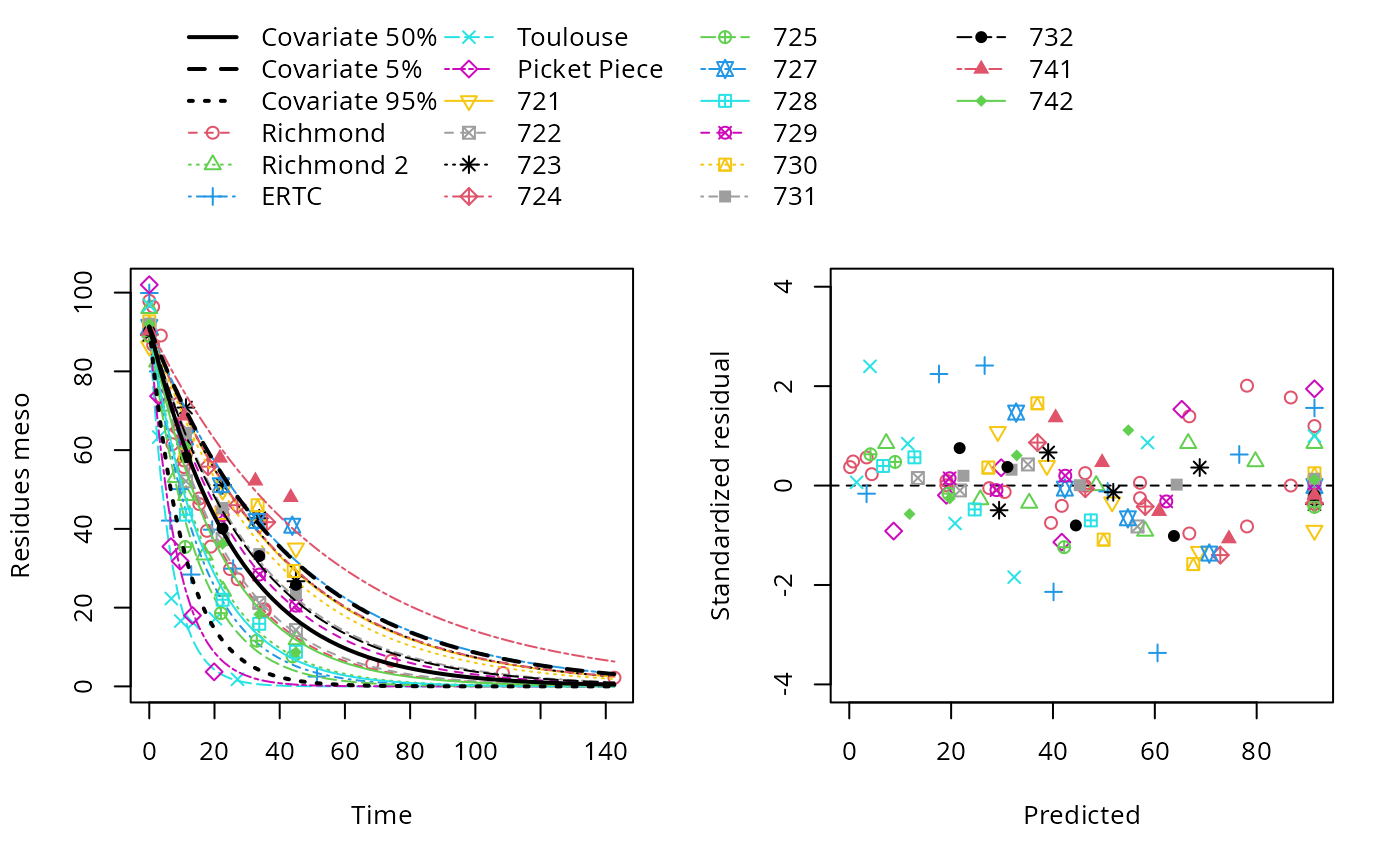

Endpoints for a model with covariates are by default calculated for the median of the covariate values. This quantile can be adapted, or a specific covariate value can be given as shown below.

endpoints(sfo_pH)

$covariates
      pH
50% 5.75

$distimes
         DT50     DT90
meso 18.52069 61.52441

endpoints(sfo_pH, covariate_quantile = 0.9)

$covariates
      pH
90% 7.13

$distimes
         DT50     DT90
meso 8.237019 27.36278

endpoints(sfo_pH, covariates = c(pH = 7.0))

$covariates
     pH
User  7

$distimes
        DT50    DT90
meso 8.89035 29.5331

FOMC

fomc_pH <- saem(f_sep_const["FOMC", ], no_random_effect = "meso_0", covariates = pH,
  covariate_models = list(log_alpha ~ pH))

summary(fomc_pH)$confint_trans |> kable(digits = 2)

	est.	lower	upper
meso_0	92.84	90.75	94.93
log_alpha	-2.21	-3.49	-0.92
beta_pH(log_alpha)	0.58	0.37	0.79
log_beta	4.21	3.44	4.99
a.1	5.03	4.32	5.73
SD.log_alpha	0.00	-23.77	23.78
SD.log_beta	0.37	0.01	0.74

As in the case of SFO, the confidence interval of the slope parameter (here beta_pH(log_alpha)) quantifying the influence of soil pH does not include zero, and the model comparison clearly indicates that the model with covariate influence is preferable. However, the random effect for alpha is not well-defined any more after inclusion of the covariate effect (the confidence interval of SD.log_alpha includes zero).

illparms(fomc_pH)

[1] "sd(log_alpha)"

Therefore, the model is updated without this random effect, and no ill-defined parameters remain.

fomc_pH_2 <- update(fomc_pH, no_random_effect = c("meso_0", "log_alpha"))
illparms(fomc_pH_2)

anova(f_saem_2[["FOMC", "const"]], fomc_pH, fomc_pH_2, test = TRUE)

Data: 116 observations of 1 variable(s) grouped in 18 datasets

                            npar    AIC    BIC     Lik  Chisq Df Pr(>Chisq)    
f_saem_2[["FOMC", "const"]]    5 783.25 787.71 -386.63                         
fomc_pH_2                      6 767.49 772.83 -377.75 17.762  1  2.503e-05 ***
fomc_pH                        7 770.07 776.30 -378.04  0.000  1          1    
---
Signif. codes:  0 '***' 0.001 '**' 0.01 '*' 0.05 '.' 0.1 ' ' 1

Model comparison indicates that including pH dependence significantly improves the fit, and that the reduced model with covariate influence results in the most preferable FOMC fit.

summary(fomc_pH_2)$confint_trans |> kable(digits = 2)

	est.	lower	upper
meso_0	93.05	90.98	95.13
log_alpha	-2.91	-4.18	-1.63
beta_pH(log_alpha)	0.66	0.44	0.87
log_beta	3.95	3.29	4.62
a.1	4.98	4.28	5.68
SD.log_beta	0.40	0.26	0.54

plot(fomc_pH_2)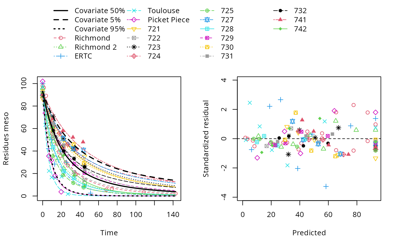

endpoints(fomc_pH_2)

$covariates
      pH
50% 5.75

$distimes
         DT50     DT90 DT50back
meso 17.30248 82.91343 24.95943

endpoints(fomc_pH_2, covariates = c(pH = 7))

$covariates
     pH
User  7

$distimes
         DT50     DT90 DT50back
meso 6.986239 27.02927 8.136621

DFOP

In the DFOP fits without covariate effects, random effects for two degradation parameters (k2 and g) were identifiable.

summary(f_saem_2[["DFOP", "const"]])$confint_trans |> kable(digits = 2)

	est.	lower	upper
meso_0	93.61	91.58	95.63
log_k1	-1.53	-2.27	-0.79
log_k2	-3.42	-3.73	-3.11
g_qlogis	-1.67	-2.57	-0.77
a.1	4.74	4.02	5.45
SD.log_k2	0.60	0.38	0.81
SD.g_qlogis	0.94	0.33	1.54

A fit with pH dependent degradation parameters was obtained by excluding the same random effects as in the refined DFOP fit without covariate influence, and including covariate models for the two identifiable parameters k2 and g.

dfop_pH <- saem(f_sep_const["DFOP", ], no_random_effect = c("meso_0", "log_k1"),
  covariates = pH,
  covariate_models = list(log_k2 ~ pH, g_qlogis ~ pH))

The corresponding parameters for the influence of soil pH are beta_pH(log_k2) for the influence of soil pH on k2, and beta_pH(g_qlogis) for its influence on g.

summary(dfop_pH)$confint_trans |> kable(digits = 2)

	est.	lower	upper
meso_0	92.84	90.85	94.84
log_k1	-2.82	-3.09	-2.54
log_k2	-11.48	-15.32	-7.64
beta_pH(log_k2)	1.31	0.69	1.92
g_qlogis	3.13	0.47	5.80
beta_pH(g_qlogis)	-0.57	-1.04	-0.09
a.1	4.96	4.26	5.65
SD.log_k2	0.76	0.47	1.05
SD.g_qlogis	0.01	-9.96	9.97

illparms(dfop_pH)

[1] "sd(g_qlogis)"

Confidence intervals for neither of them include zero, indicating a significant difference from zero. However, the random effect for g is now ill-defined. The fit is updated without this ill-defined random effect.

dfop_pH_2 <- update(dfop_pH,
  no_random_effect = c("meso_0", "log_k1", "g_qlogis"))
illparms(dfop_pH_2)

[1] "beta_pH(g_qlogis)"

Now, the slope parameter for the pH effect on g is ill-defined. Therefore, another attempt is made without the corresponding covariate model.

dfop_pH_3 <- saem(f_sep_const["DFOP", ], no_random_effect = c("meso_0", "log_k1"),
  covariates = pH,
  covariate_models = list(log_k2 ~ pH))
illparms(dfop_pH_3)

[1] "sd(g_qlogis)"

As the random effect for g is again ill-defined, the fit is repeated without it.

dfop_pH_4 <- update(dfop_pH_3, no_random_effect = c("meso_0", "log_k1", "g_qlogis"))
illparms(dfop_pH_4)

While no ill-defined parameters remain, model comparison suggests that the previous model dfop_pH_2 with two pH dependent parameters is preferable, based on information criteria as well as based on the likelihood ratio test.

anova(f_saem_2[["DFOP", "const"]], dfop_pH, dfop_pH_2, dfop_pH_3, dfop_pH_4)

Data: 116 observations of 1 variable(s) grouped in 18 datasets

                            npar    AIC    BIC     Lik
f_saem_2[["DFOP", "const"]]    7 782.94 789.18 -384.47
dfop_pH_4                      7 767.35 773.58 -376.68
dfop_pH_2                      8 765.14 772.26 -374.57
dfop_pH_3                      8 769.00 776.12 -376.50
dfop_pH                        9 769.10 777.11 -375.55

anova(dfop_pH_2, dfop_pH_4, test = TRUE)

Data: 116 observations of 1 variable(s) grouped in 18 datasets

          npar    AIC    BIC     Lik  Chisq Df Pr(>Chisq)  
dfop_pH_4    7 767.35 773.58 -376.68                       
dfop_pH_2    8 765.14 772.26 -374.57 4.2153  1    0.04006 *
---
Signif. codes:  0 '***' 0.001 '**' 0.01 '*' 0.05 '.' 0.1 ' ' 1

When focussing on parameter identifiability using the test if the confidence interval includes zero, dfop_pH_4 would still be the preferred model. However, it should be kept in mind that parameter confidence intervals are constructed using a simple linearisation of the likelihood. As the confidence interval of the random effect for g only marginally includes zero, it is suggested that this is acceptable, and that dfop_pH_2 can be considered the most preferable model.

plot(dfop_pH_2)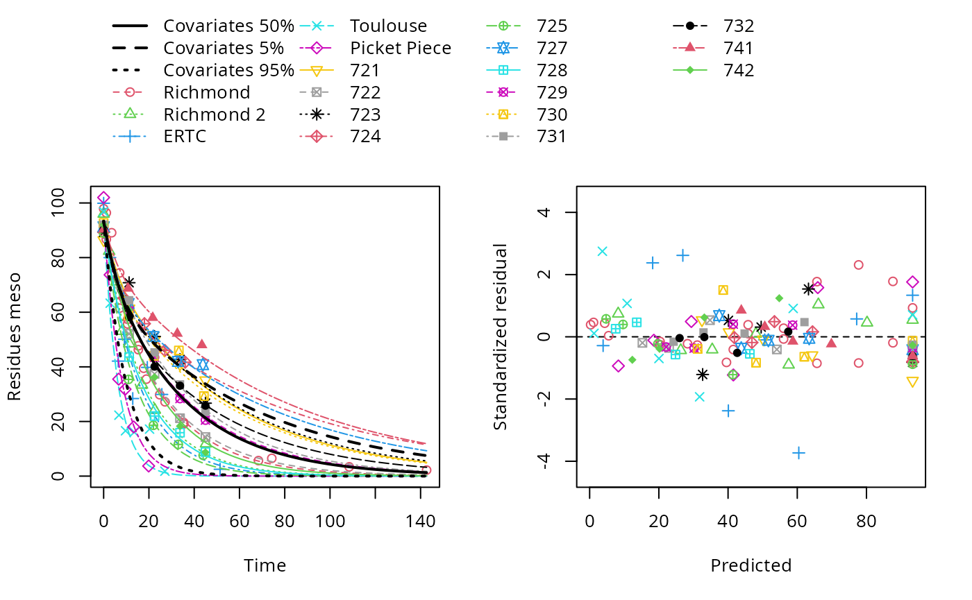

endpoints(dfop_pH_2)

$covariates
      pH
50% 5.75

$distimes
         DT50     DT90 DT50back  DT50_k1  DT50_k2
meso 18.36876 73.51841 22.13125 4.191901 23.98672

endpoints(dfop_pH_2, covariates = c(pH = 7))

$covariates
     pH
User  7

$distimes
         DT50     DT90 DT50back  DT50_k1  DT50_k2
meso 8.346428 28.34437 8.532507 4.191901 8.753618

SFORB

sforb_pH <- saem(f_sep_const["SFORB", ], no_random_effect = c("meso_free_0", "log_k_meso_free_bound"),
  covariates = pH,
  covariate_models = list(log_k_meso_free ~ pH, log_k_meso_bound_free ~ pH))

summary(sforb_pH)$confint_trans |> kable(digits = 2)

	est.	lower	upper
meso_free_0	93.42	91.32	95.52
log_k_meso_free	-5.37	-6.94	-3.81
beta_pH(log_k_meso_free)	0.42	0.18	0.67
log_k_meso_free_bound	-3.49	-4.92	-2.05
log_k_meso_bound_free	-9.98	-19.22	-0.74
beta_pH(log_k_meso_bound_free)	1.23	-0.21	2.67
a.1	4.90	4.18	5.63
SD.log_k_meso_free	0.35	0.23	0.47
SD.log_k_meso_bound_free	0.13	-1.95	2.20

The confidence interval of beta_pH(log_k_meso_bound_free) includes zero, indicating that the influence of soil pH on k_meso_bound_free cannot reliably be quantified. Also, the confidence interval for the random effect on this parameter (SD.log_k_meso_bound_free) includes zero.

Using the illparms function, these ill-defined parameters can be found more conveniently.

illparms(sforb_pH)

[1] "sd(log_k_meso_bound_free)"      "beta_pH(log_k_meso_bound_free)"

To remove the ill-defined parameters, a second variant of the SFORB model with pH influence is fitted. No ill-defined parameters remain.

sforb_pH_2 <- update(sforb_pH,
  no_random_effect = c("meso_free_0", "log_k_meso_free_bound", "log_k_meso_bound_free"),
  covariate_models = list(log_k_meso_free ~ pH))
illparms(sforb_pH_2)

The model comparison of the SFORB fits includes the refined model without covariate effect, and both versions of the SFORB fit with covariate effect.

anova(f_saem_2[["SFORB", "const"]], sforb_pH, sforb_pH_2, test = TRUE)

Data: 116 observations of 1 variable(s) grouped in 18 datasets

                             npar    AIC    BIC     Lik   Chisq Df Pr(>Chisq)  
f_saem_2[["SFORB", "const"]]    7 783.40 789.63 -384.70                        
sforb_pH_2                      7 770.94 777.17 -378.47 12.4616  0             
sforb_pH                        9 768.81 776.83 -375.41  6.1258  2    0.04675 *
---
Signif. codes:  0 '***' 0.001 '**' 0.01 '*' 0.05 '.' 0.1 ' ' 1

The first model including pH influence is preferable based on information criteria and the likelihood ratio test. However, as it is not fully identifiable, the second model is selected.

summary(sforb_pH_2)$confint_trans |> kable(digits = 2)

	est.	lower	upper
meso_free_0	93.32	91.16	95.48
log_k_meso_free	-6.15	-7.43	-4.86
beta_pH(log_k_meso_free)	0.54	0.33	0.75
log_k_meso_free_bound	-3.80	-5.20	-2.40
log_k_meso_bound_free	-2.95	-4.26	-1.64
a.1	5.08	4.38	5.79
SD.log_k_meso_free	0.33	0.22	0.45

plot(sforb_pH_2)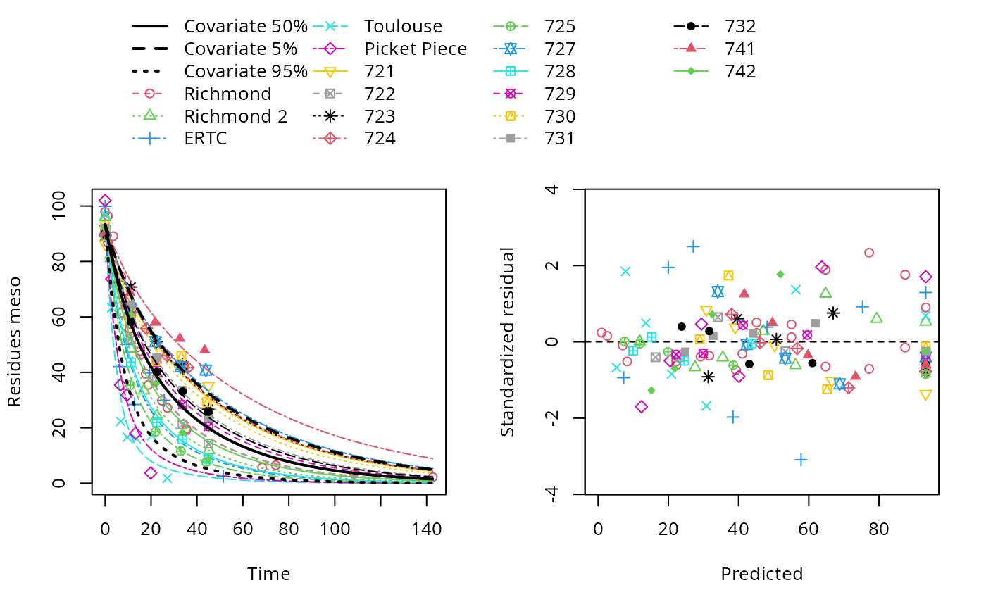

endpoints(sforb_pH_2)

$covariates
      pH
50% 5.75

$ff
meso_free 
        1 

$SFORB
   meso_b1    meso_b2     meso_g 
0.09735824 0.02631699 0.31602120 

$distimes
         DT50     DT90 DT50back DT50_meso_b1 DT50_meso_b2
meso 16.86549 73.15824 22.02282     7.119554     26.33839

endpoints(sforb_pH_2, covariates = c(pH = 7))

$covariates
     pH
User  7

$ff
meso_free 
        1 

$SFORB
   meso_b1    meso_b2     meso_g 
0.13315233 0.03795988 0.61186191 

$distimes
         DT50     DT90 DT50back DT50_meso_b1 DT50_meso_b2
meso 7.932495 36.93311 11.11797     5.205671        18.26

HS

hs_pH <- saem(f_sep_const["HS", ], no_random_effect = c("meso_0"),
  covariates = pH,
  covariate_models = list(log_k1 ~ pH, log_k2 ~ pH, log_tb ~ pH))

summary(hs_pH)$confint_trans |> kable(digits = 2)

	est.	lower	upper
meso_0	93.33	91.47	95.19
log_k1	-5.81	-7.27	-4.36
beta_pH(log_k1)	0.47	0.23	0.72
log_k2	-6.80	-8.76	-4.83
beta_pH(log_k2)	0.54	0.21	0.87
log_tb	3.25	1.25	5.25
beta_pH(log_tb)	-0.10	-0.43	0.23
a.1	4.49	3.78	5.21
SD.log_k1	0.37	0.24	0.51
SD.log_k2	0.29	0.10	0.48
SD.log_tb	0.25	-0.07	0.57

illparms(hs_pH)

[1] "sd(log_tb)"      "beta_pH(log_tb)"

According to the output of the illparms function, the random effect on the break time tb cannot reliably be quantified, neither can the influence of soil pH on tb. The fit is repeated without the corresponding covariate model, and no ill-defined parameters remain.

hs_pH_2 <- update(hs_pH, covariate_models = list(log_k1 ~ pH, log_k2 ~ pH))
illparms(hs_pH_2)

Model comparison confirms that this model is preferable to the fit without covariate influence, and also to the first version with covariate influence.

anova(f_saem_2[["HS", "const"]], hs_pH, hs_pH_2, test = TRUE)

Data: 116 observations of 1 variable(s) grouped in 18 datasets

                          npar    AIC    BIC     Lik  Chisq Df Pr(>Chisq)    
f_saem_2[["HS", "const"]]    8 780.08 787.20 -382.04                         
hs_pH_2                     10 766.47 775.37 -373.23 17.606  2  0.0001503 ***
hs_pH                       11 769.80 779.59 -373.90  0.000  1  1.0000000    
---
Signif. codes:  0 '***' 0.001 '**' 0.01 '*' 0.05 '.' 0.1 ' ' 1

summary(hs_pH_2)$confint_trans |> kable(digits = 2)

	est.	lower	upper
meso_0	93.33	91.50	95.15
log_k1	-5.68	-7.09	-4.27
beta_pH(log_k1)	0.46	0.22	0.69
log_k2	-6.61	-8.34	-4.88
beta_pH(log_k2)	0.50	0.21	0.79
log_tb	2.70	2.33	3.08
a.1	4.45	3.74	5.16
SD.log_k1	0.36	0.22	0.49
SD.log_k2	0.23	0.02	0.43
SD.log_tb	0.55	0.25	0.85

plot(hs_pH_2)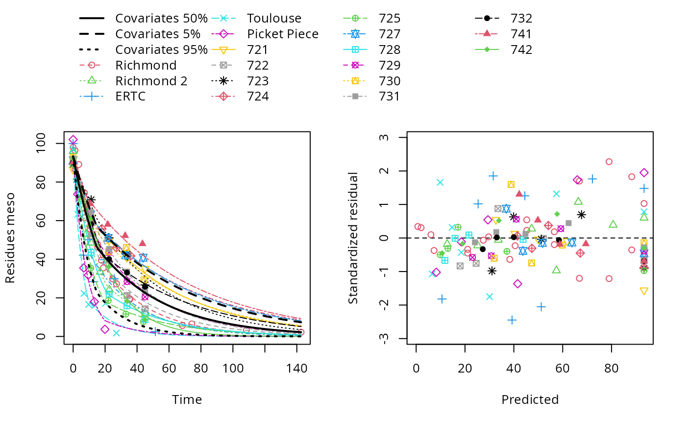

endpoints(hs_pH_2)

$covariates
      pH
50% 5.75

$distimes
         DT50     DT90 DT50back  DT50_k1  DT50_k2
meso 14.68725 82.45287 24.82079 14.68725 29.29299

endpoints(hs_pH_2, covariates = c(pH = 7))

$covariates
     pH
User  7

$distimes
         DT50     DT90 DT50back  DT50_k1  DT50_k2
meso 8.298536 38.85371 11.69613 8.298536 15.71561

Comparison across parent models

After model reduction for all models with pH influence, they are compared with each other.

anova(sfo_pH, fomc_pH_2, dfop_pH_2, dfop_pH_4, sforb_pH_2, hs_pH_2)

Data: 116 observations of 1 variable(s) grouped in 18 datasets

           npar    AIC    BIC     Lik
sfo_pH        5 783.09 787.54 -386.54
fomc_pH_2     6 767.49 772.83 -377.75
dfop_pH_4     7 767.35 773.58 -376.68
sforb_pH_2    7 770.94 777.17 -378.47
dfop_pH_2     8 765.14 772.26 -374.57
hs_pH_2      10 766.47 775.37 -373.23

The DFOP model with pH influence on k2 and g and a random effect only on k2 is finally selected as the best fit.

The endpoints resulting from this model are listed below. Please refer to the Appendix for a detailed listing.

endpoints(dfop_pH_2)

$covariates
      pH
50% 5.75

$distimes
         DT50     DT90 DT50back  DT50_k1  DT50_k2
meso 18.36876 73.51841 22.13125 4.191901 23.98672

endpoints(dfop_pH_2, covariates = c(pH = 7))

$covariates
     pH
User  7

$distimes
         DT50     DT90 DT50back  DT50_k1  DT50_k2
meso 8.346428 28.34437 8.532507 4.191901 8.753618

Conclusions

These evaluations demonstrate that covariate effects can be included for all types of parent degradation models. These models can then be further refined to make them fully identifiable.

Appendix

Hierarchical fit listings

Fits without covariate effects

Fits with covariate effects

Session info

R version 4.3.2 (2023-10-31)
Platform: x86_64-pc-linux-gnu (64-bit)
Running under: Debian GNU/Linux 12 (bookworm)

Matrix products: default
BLAS:   /usr/lib/x86_64-linux-gnu/blas/libblas.so.3.11.0 
LAPACK: /usr/lib/x86_64-linux-gnu/lapack/liblapack.so.3.11.0

locale:
 [1] LC_CTYPE=de_DE.UTF-8       LC_NUMERIC=C              
 [3] LC_TIME=de_DE.UTF-8        LC_COLLATE=de_DE.UTF-8    
 [5] LC_MONETARY=de_DE.UTF-8    LC_MESSAGES=de_DE.UTF-8   
 [7] LC_PAPER=de_DE.UTF-8       LC_NAME=C                 
 [9] LC_ADDRESS=C               LC_TELEPHONE=C            
[11] LC_MEASUREMENT=de_DE.UTF-8 LC_IDENTIFICATION=C       

time zone: Europe/Berlin
tzcode source: system (glibc)

attached base packages:
[1] parallel  stats     graphics  grDevices utils     datasets  methods  
[8] base     

other attached packages:
[1] saemix_3.2 npde_3.3   knitr_1.42 mkin_1.2.6

loaded via a namespace (and not attached):
 [1] sass_0.4.6        utf8_1.2.3        generics_0.1.3    stringi_1.7.12   
 [5] lattice_0.21-8    digest_0.6.31     magrittr_2.0.3    evaluate_0.21    
 [9] grid_4.3.2        fastmap_1.1.1     rprojroot_2.0.3   jsonlite_1.8.4   
[13] DBI_1.1.3         mclust_6.0.0      gridExtra_2.3     purrr_1.0.1      
[17] fansi_1.0.4       scales_1.2.1      textshaping_0.3.6 jquerylib_0.1.4  
[21] cli_3.6.1         rlang_1.1.1       munsell_0.5.0     cachem_1.0.8     
[25] yaml_2.3.7        tools_4.3.2       memoise_2.0.1     dplyr_1.1.2      
[29] colorspace_2.1-0  ggplot2_3.4.2     vctrs_0.6.2       R6_2.5.1         
[33] zoo_1.8-12        lifecycle_1.0.3   stringr_1.5.0     fs_1.6.2         
[37] MASS_7.3-60       ragg_1.2.5        pkgconfig_2.0.3   desc_1.4.2       
[41] pkgdown_2.0.7     bslib_0.4.2       pillar_1.9.0      gtable_0.3.3     
[45] glue_1.6.2        systemfonts_1.0.4 xfun_0.39         tibble_3.2.1     
[49] lmtest_0.9-40     tidyselect_1.2.0  htmltools_0.5.5   nlme_3.1-163     
[53] rmarkdown_2.21    compiler_4.3.2

Hardware info

CPU model: AMD Ryzen 9 7950X 16-Core Processor

MemTotal:       64928100 kB

Johannes Ranke

Last change on 4 August 2023, last compiled on 16 November 2023